ICCP 2026 Summer School
Interferometric Imaging
Build a Michelson-style interferometer on a breadboard, align it to see white-light interference fringes, and use it as a time-domain OCT scanner to recover a depth map of a coin.
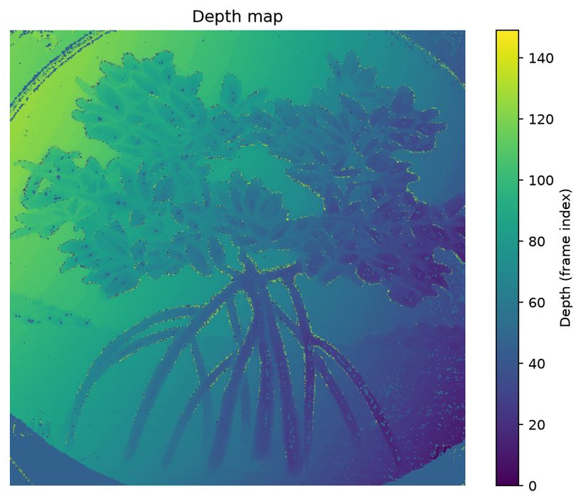
Where this is going: by the end of this guide you will have built a scanner that can map a surface down to micron scale — the depth map below, and the transient video of the coherence gate sweeping across a coin, are both produced by the instrument you're about to build.
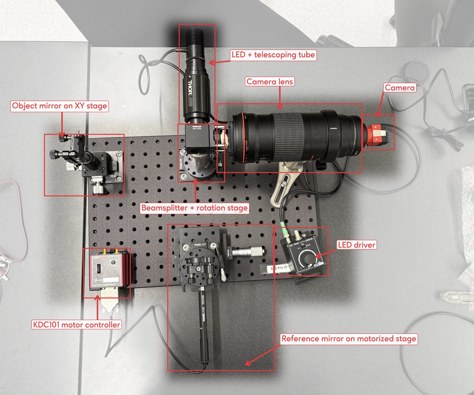
The setup you will build — a Michelson interferometer on a breadboard. Light from the LED is split at the beamsplitter into two arms — the reference mirror on the motorized stage, and the object (a mirror at first, later your coin) on the XY stage — and recombines into the camera:
The results — what this instrument measures:
Construction
1Start with the breadboard
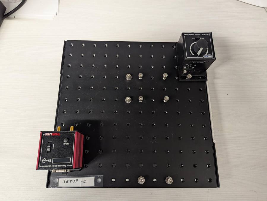
Your breadboard should look something like this — the LED driver (red box) and the LED mount are already in place:
2Mount the beamsplitter post
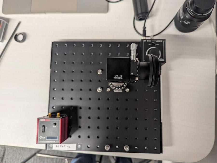
Mount the main post with the beamsplitter (BS) using the cap screws at the designated location on the breadboard. Depending on your specific setup, the position of the beamsplitter may not match the one shown below. Ask one of us to verify if the positioning is correct.
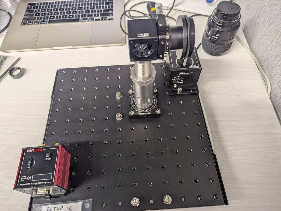
3Light source arm
- Screw on the 100 mm Thorlabs lens (AC254-100-A-ML).
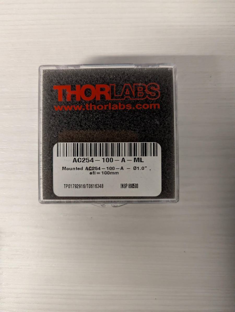
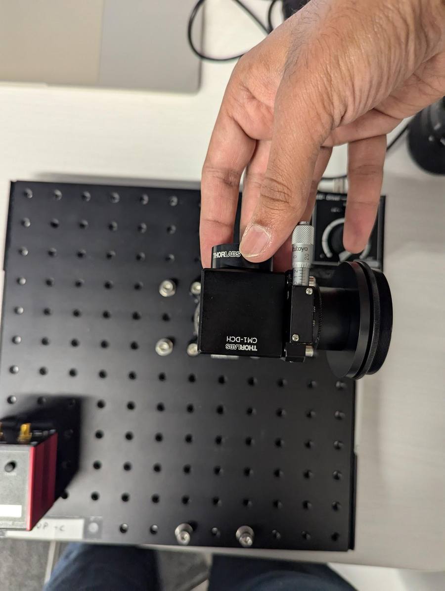
- Screw on the LED with the telescoping tube onto the threading of the lens.
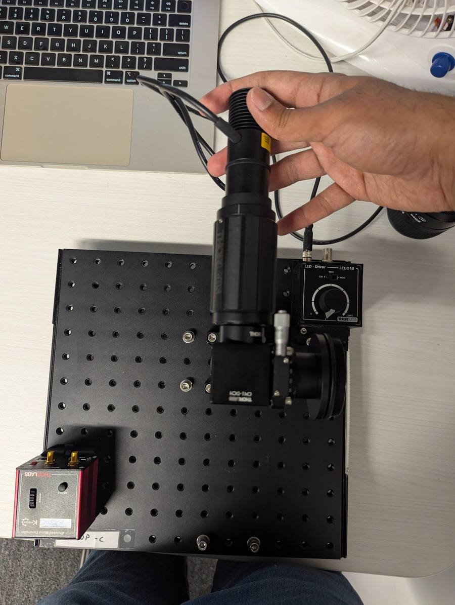
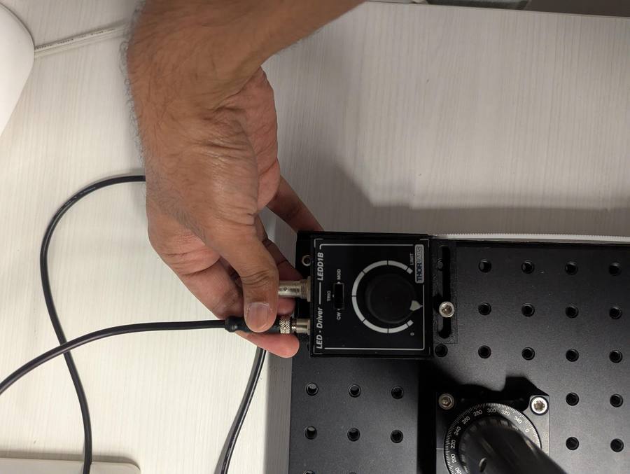
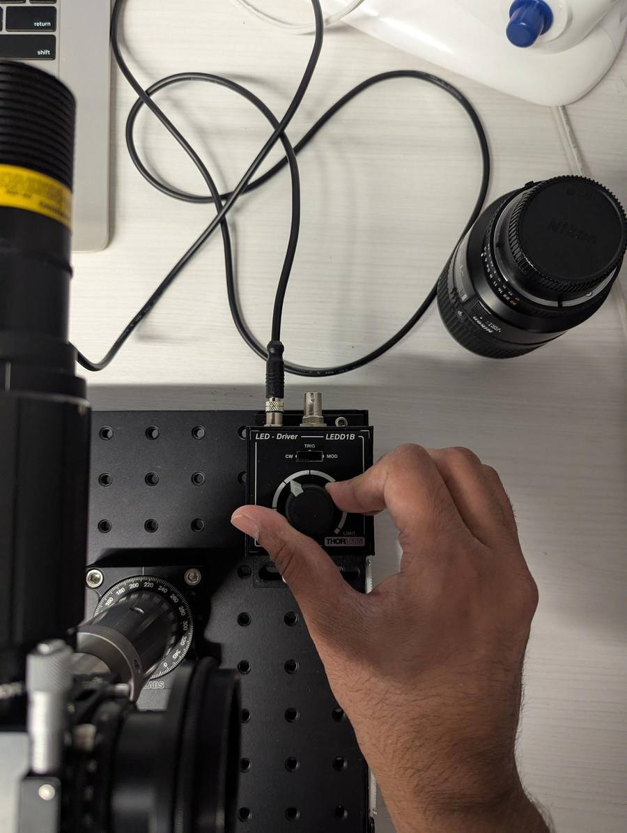
- Connect the LED to the LED driver, and try powering it up with the power adapter.
Careful: the LED can be very bright — try not to look directly into it. Turn the driver's power knob down before switching it on.
4Camera arm
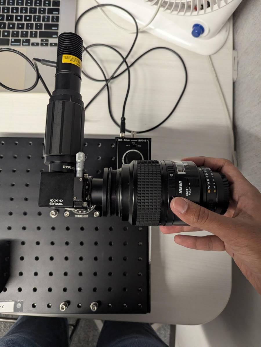
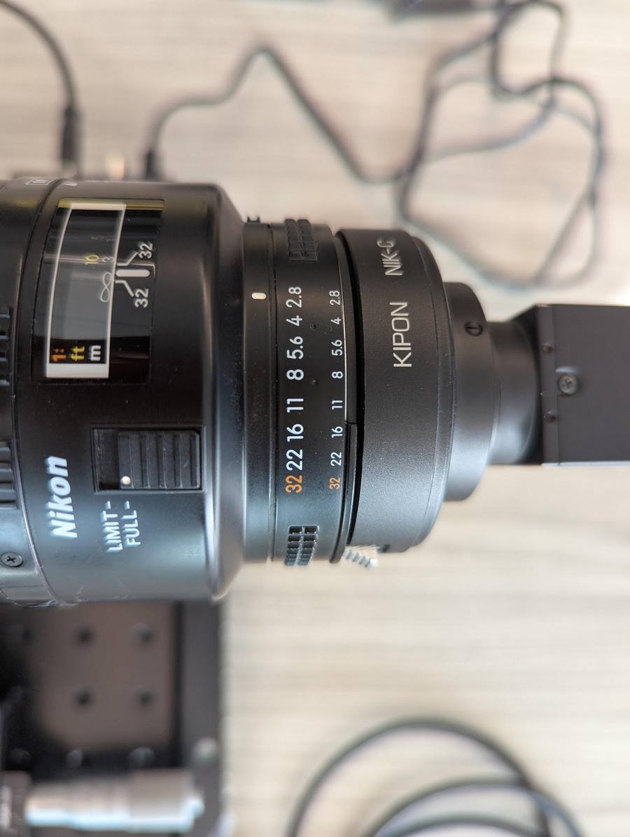
- Screw the 105 mm (or 200 mm) Nikon lens on the threading at the right end of the BS cube.
- You should have a C-mount camera that looks like this:
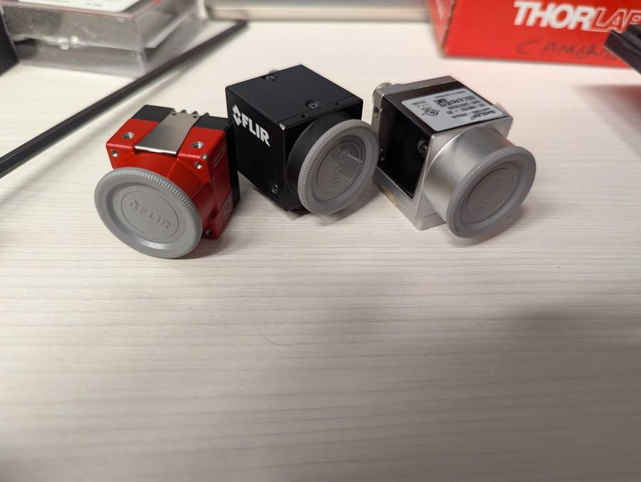
- Screw the C-mount camera onto the F-C mount, and then attach it to the back of the lens.
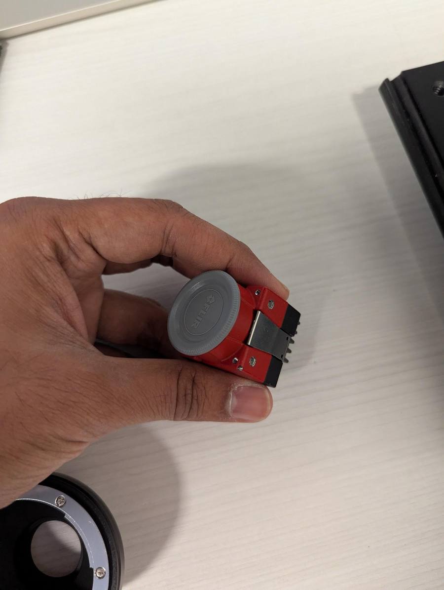
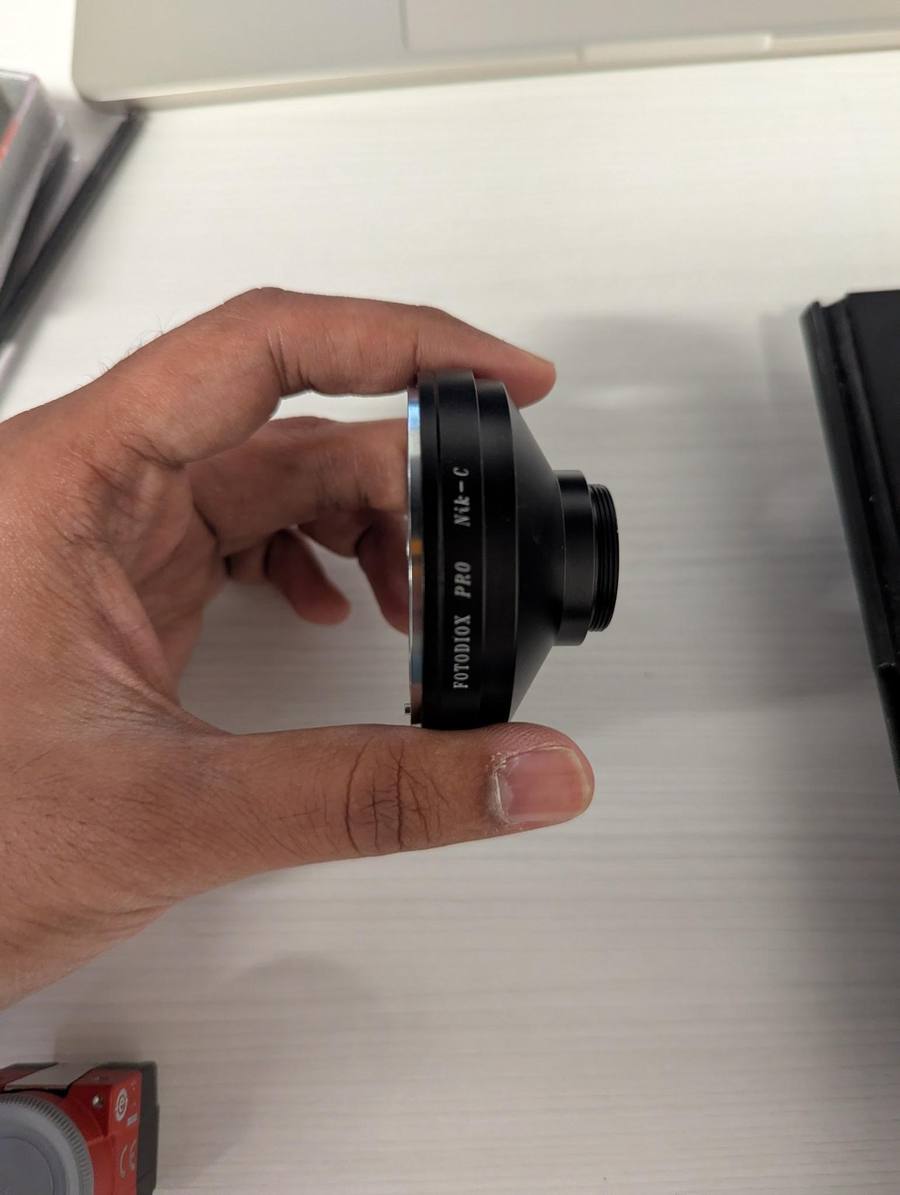
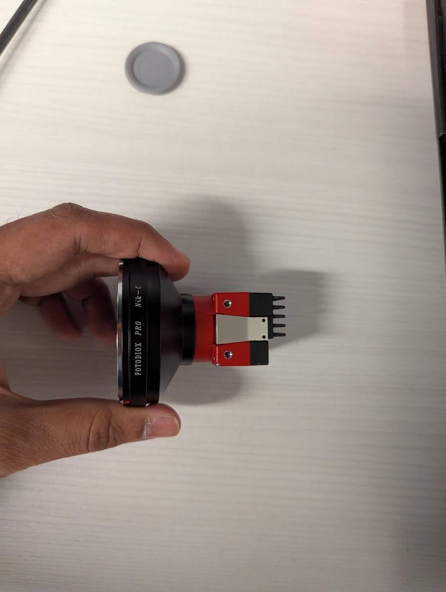
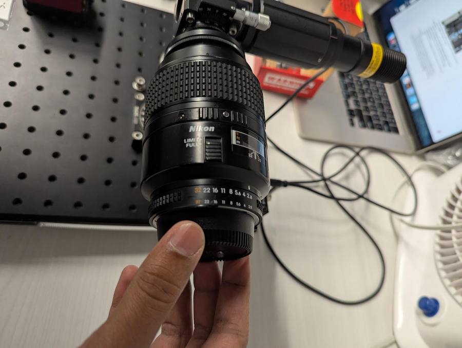
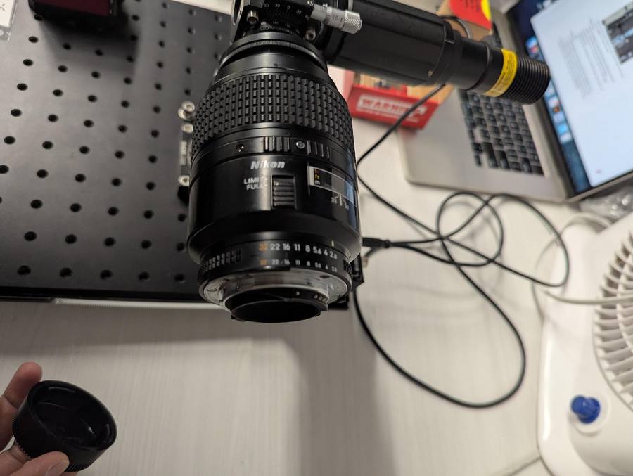 Careful: careful not to leave bare sensor open too long while handling the camera (to prevent dust/damage).
5Reference arm
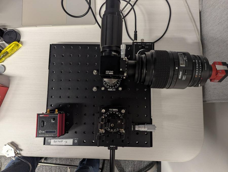
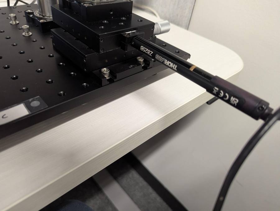
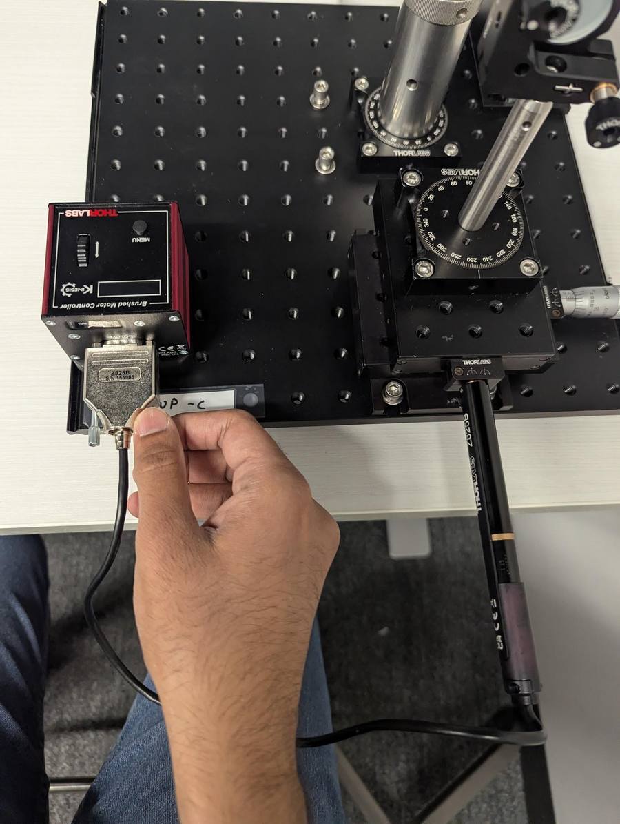
- Place the XY stage (with the motorized Z825B actuator inserted) on
the breadboard (at the designated location indicated by screws) and secure it using washers and cap screws.
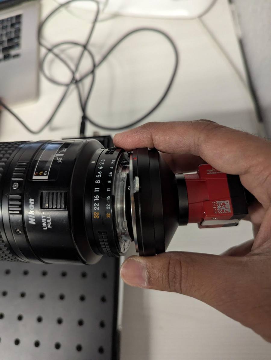
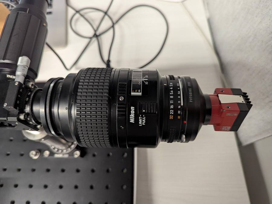
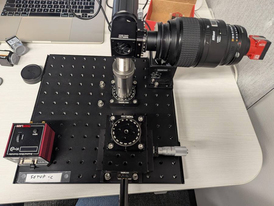
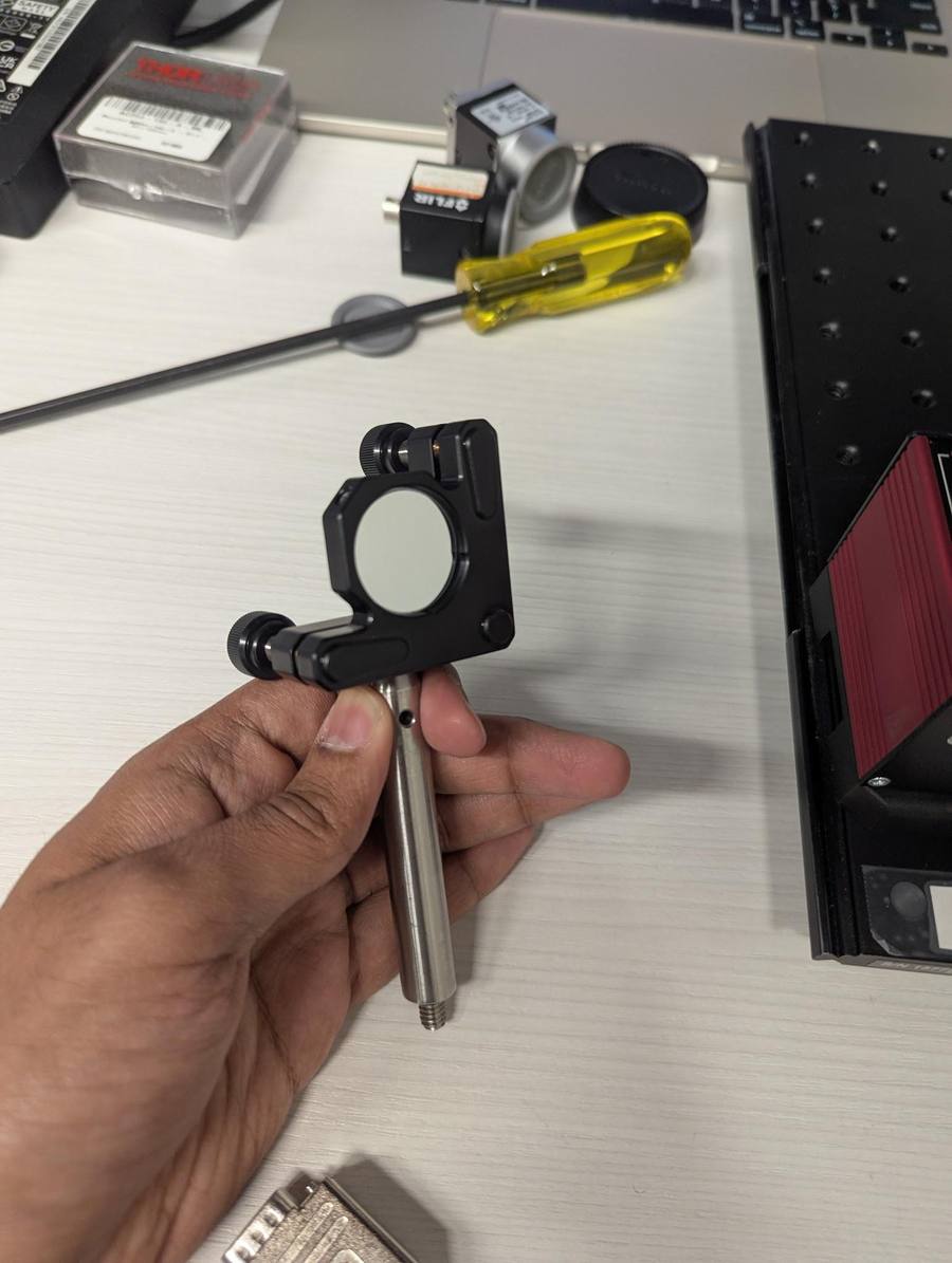
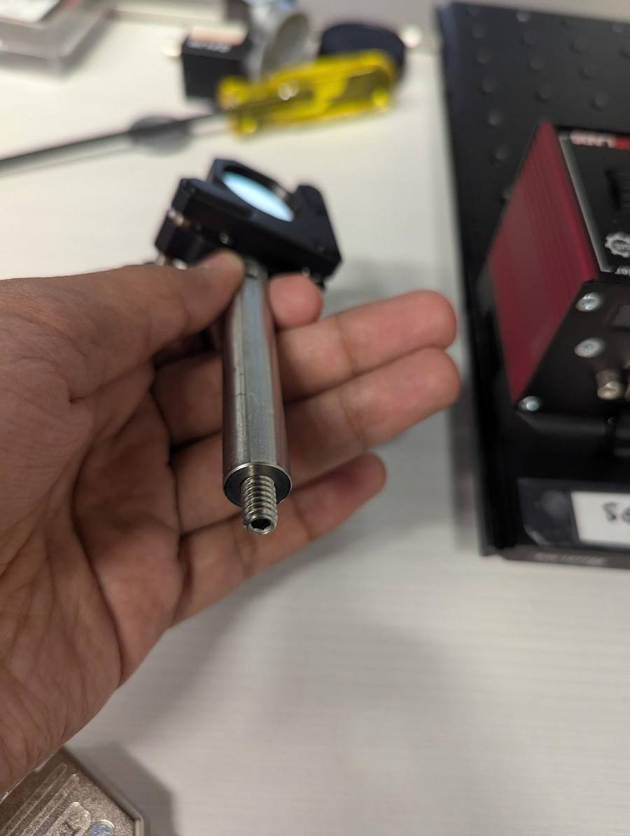
- Careful not to touch or damage the mirror — screw the round mirror mount onto the
stage using the set screw at the bottom.
- Connect the end of the Z825B motor to the KDC101 K-cube motor controller (red cube).
6Object arm
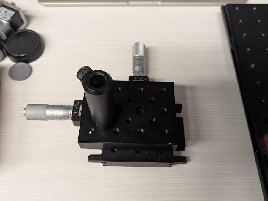
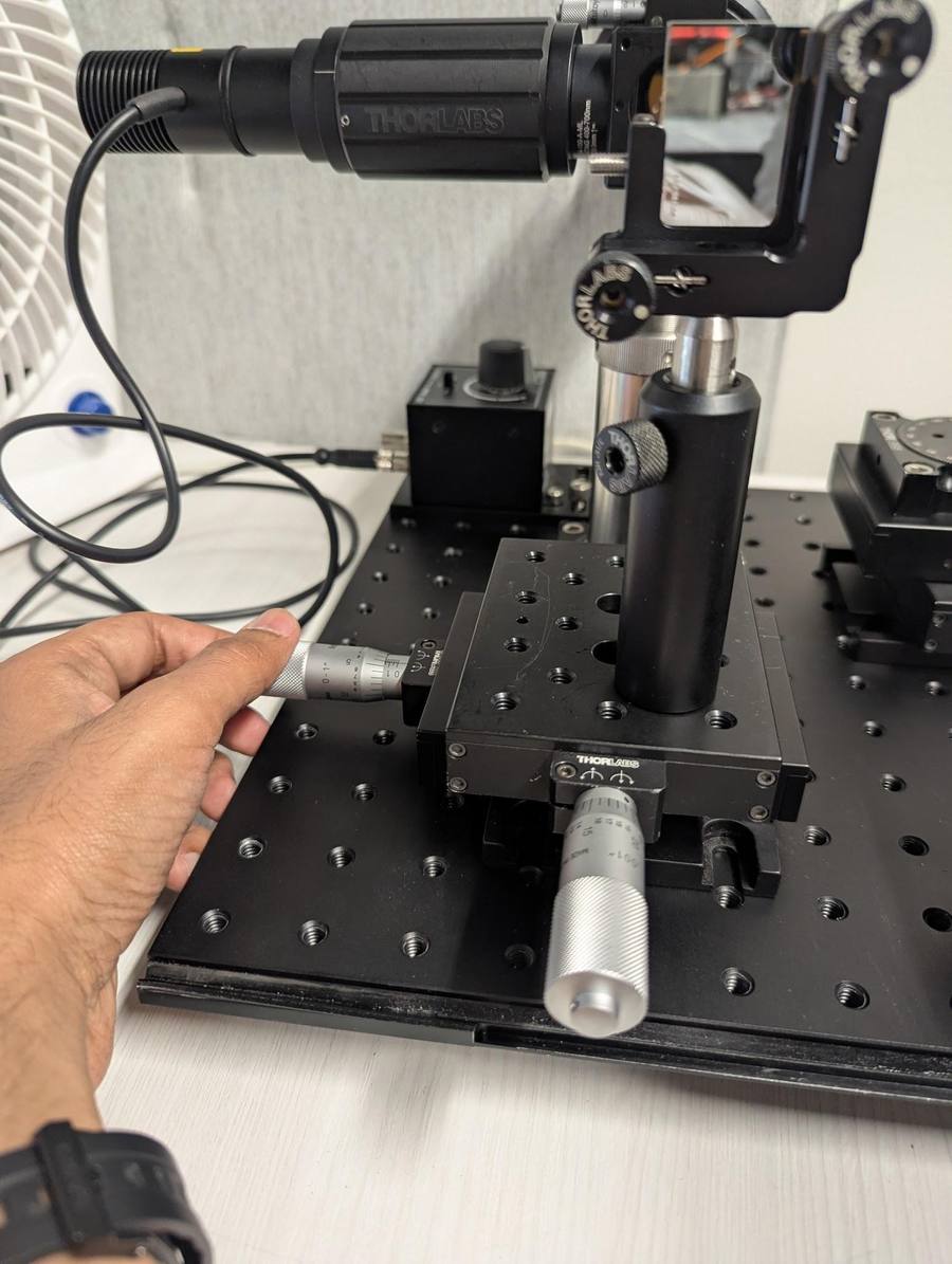
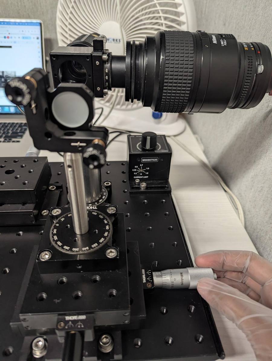
- Similar to the reference arm, place and secure the XY translation stage for the object side
at the designated location. Your stage may look slightly different from the XY stage in the image.
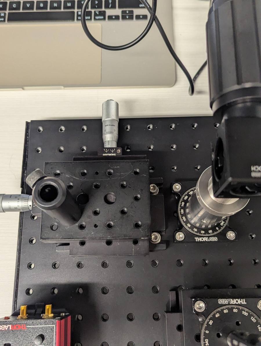
- Drop in the post holding the rectangular mirror, careful not to touch or damage the
mirror.
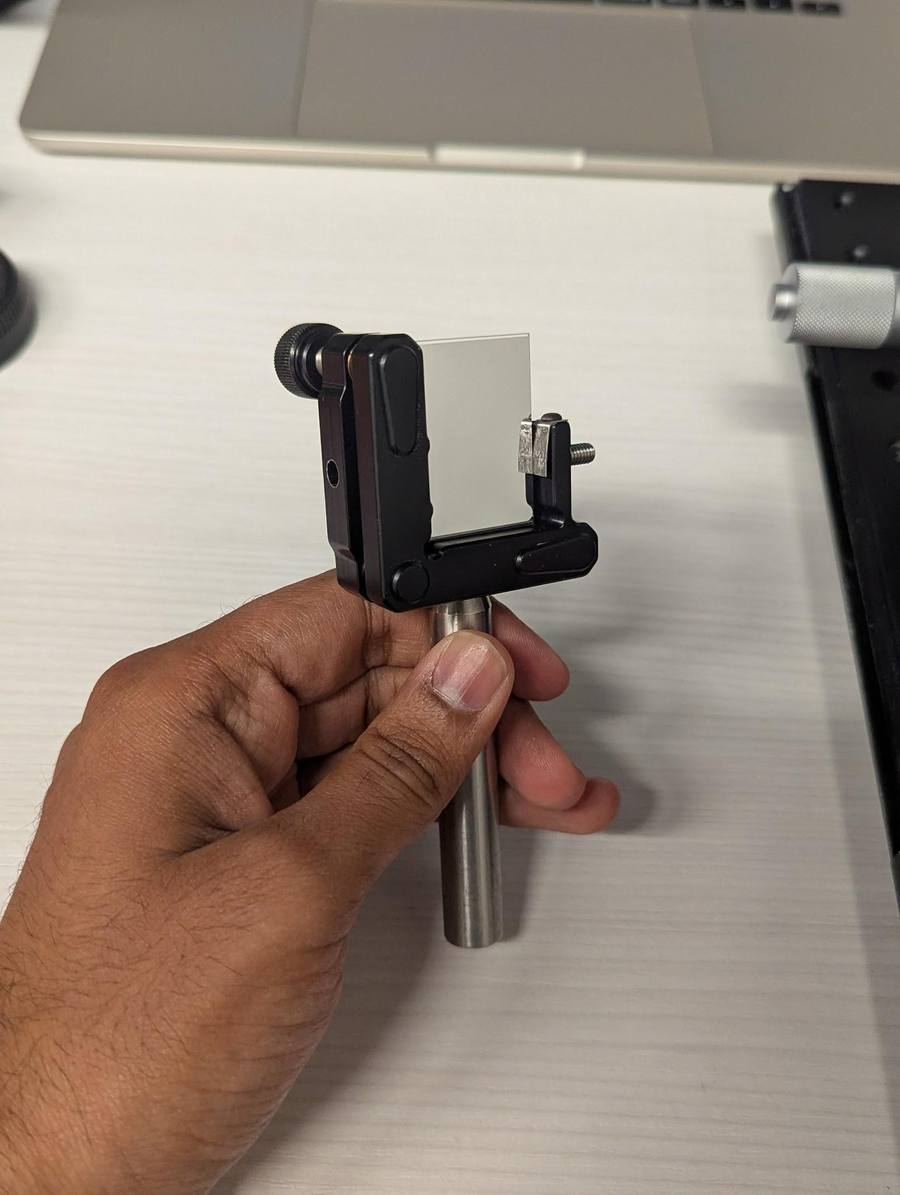
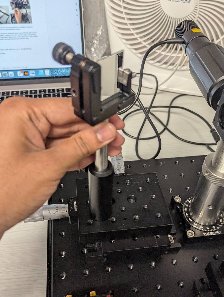
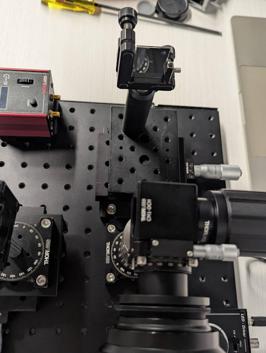
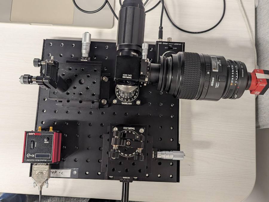
- Use the lateral micro-adjusters to position the mirrors to be facing directly opposite
the cage-cube opening.
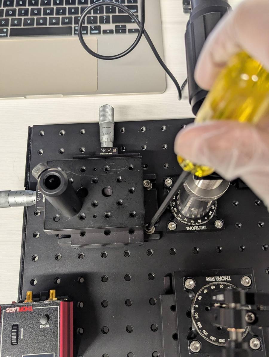
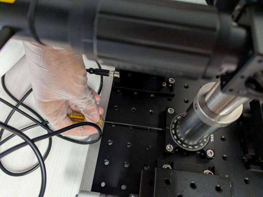
7Fix the base rotation stage
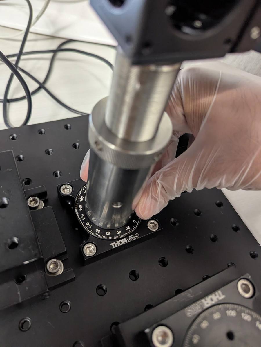
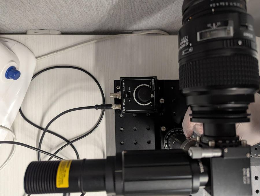
Fix the orientation of the base rotation stage at the centre (ask for a 5/64 hex key) such that the LED and camera are roughly along the breadboard holes.
Alignment
Everything in this part runs from the Python scripts in
this repository, inside the
conda environment from environment.yml.
1Hardware sanity check
Before touching any optics, make sure the laptop can actually talk to the stage and the camera. Plug in the KDC101's USB cable, switch it on with the red switch, connect the camera's USB cable, then run:
# one-time setup (see Software installations below for details)
git clone https://github.com/cmu-ci-lab/summer-school.git
cd summer-school
Then build the Python environment. Pick one of the three options below (see Software installations for the full details):
Option 1 — Recommended
Let the script decide (conda if you have it, else a .venv):
./setup.shOption 2 — Don't want conda?
Force a plain .venv, even if conda is installed:
FORCE_VENV=1 ./setup.shOption 3 — Manual conda
Skip the script and build the env yourself (needs conda):
conda env create -f environment.ymlThen activate the environment. Which command you use depends on which kind of
environment setup.sh built — it prints the right one when it finishes
(conda is preferred when you have it; otherwise it creates a .venv):
Got conda? — setup.sh made a conda env:
conda activate iccp-octNo conda? — setup.sh made a .venv:
source .venv/bin/activate
# Windows: .venv\Scripts\activatepython? If a script fails with
ModuleNotFoundError (pylablib, cv2, ...), you are probably running the wrong Python.
The repo ships a ./python wrapper (already executable) that always resolves the project
environment — just prefix any command with ./, e.g. ./python visualizer.py.
Equivalently, roll your own symlink with the environment active:
ln -sf "$CONDA_PREFIX/bin/python" python — see
Troubleshooting.After the environment is built, install the camera SDK — this is a separate step
that environment.yml doesn't cover, and which one you need depends on the camera on your
rig: the Vimba X SDK (vmbpy wheel) for Allied Vision, or the IDS Software Suite plus
pyueye for IDS uEye — note that IDS cameras work on Windows only (the
IDS Software Suite has no macOS support), so pair IDS rigs with a Windows laptop. See
Software installations below for step-by-step instructions.
With the environment active and the SDK in place, verify stage and camera connectivity:
python test_hardware.pyOr, to skip a vendor you don't have: python test_hardware.py --camera ids (IDS only —
skips the Vimba X check) or --camera avt (Allied Vision only).
pip install the vmbpy package. test_hardware.py will
automatically prompt you with instructions to do so.The stage test connects, reads the position, moves +5 mm and back, and verifies
the readback — so make sure the stage has 5 mm of clearance before you run it. The camera test
connects, grabs a frame, buffers three more, and writes a small stack to test_captures/.
What passing looks like — each step prints a checkmark as it succeeds; a healthy run looks like this:
  TEST: Stage (Thorlabs KDC101)
✓ Imported ThorlabsStage
✓ Connected to stage
✓ Read initial position: 0.000 mm
✓ Moved to 5.000 mm
✓ Position verified: 5.000 mm (error: 0.001 mm)
✓ Moved back to initial position
✓✓✓ Stage test PASSED

  TEST: Camera (IDS)
✓ Connected to camera
✓ Captured frame: shape=(2076, 3088), dtype=uint16
✓ Captured 3 frames to buffer
✓ Saved stack: test_captures/test_stack.npy (36.6 MB)
✓✓✓ Camera test PASSED

  SUMMARY
  Stage:  ✓ PASS
  Camera: ✓ PASS
Things to check in that output beyond the checkmarks:
- Position error — after the +5 mm move, the test reads the stage's own encoder back and compares it with the commanded target; the difference should be well under 0.1 mm. You'll essentially never see it fail — a ⚠ warning here usually just means the readback happened before the motion fully settled, or (rarely) the wrong stage model was auto-detected.
- Frame shape and dtype should match your sensor — full resolution, and
uint16if the camera runs a 10/12-bit mode (IDS) rather than 8-bit. - The saved stack size should be plausible (a few frames × resolution × 1–2 bytes).
libusb must be installed). If a script crashed earlier, the hardware may still be held
by its Python kernel — restart the kernel and retry. A camera failure is usually a missing vendor SDK;
the script prints exactly which package to install (e.g. the vmbpy wheel from
Vimba X).2Getting light into the camera
- Ensure the lens aperture is fully open.
- Launch the visualizer — everything in the rest of this part happens inside it. It auto-detects
the camera (AVT or IDS), connects to the stage, and homes it on startup:
# live camera preview + coherence panel
# --step: coarse stage step in mm; --window-mm: positional window for the DC mean
python visualizer.py --step 0.01 --window-mm 0.2
Stage control: the reference stage is driven from the keyboard — w/s jog by the coarse step, e/d by the fine step (coarse ÷ 10), and [/] change the step size. To sweep, just hold w or e — the stage moves continuously; there is no need for slow individual presses. The status bar along the bottom shows exposure, frame rate, the current stage position, and the step sizes.Don't sweep backwards: the backward keys s/d produce a mechanical kick-back when the stage reverses direction (backlash). Use them only to reposition; always take your measurement sweeps forward with w/e.Ignore the coherence panel for now — the plot and stat tiles on the right of the window aren't needed until Section 3 (OCT). In this section you only use the live image and the stage keys. - Adjust your camera to be roughly upright by rotating it about the rotation mount with graduations.
videoRotating the camera about the graduated rotation mount until the image is upright. - Switch on the LED (careful — it can be very bright; avoid looking directly into it), and try to
coarsely align the orientation of the mirrors to get maximum light
into the camera by:
- coarsely adjusting the mirror post mounts,
- using the mirror adjuster knobs.
videoThe mirror adjuster knobs on the kinematic mount — these tilt the mirror to steer its image of the LED. You should see two ‘blobs’ — (likely blurred) images of the LED — that move as you adjust the mirrors.
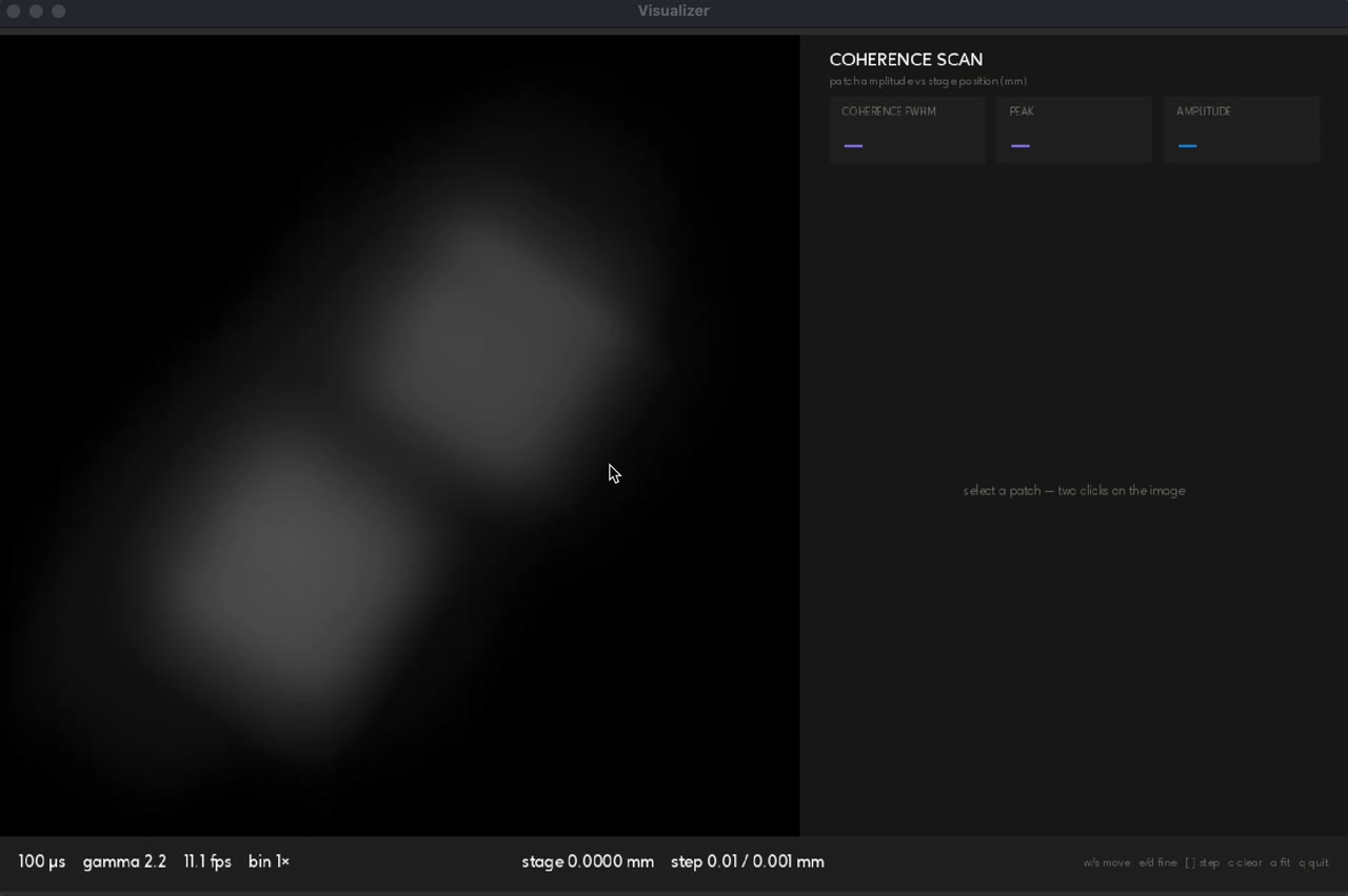
The visualizer with the two (blurred) images of the LED in the live view — coherence panel still empty on the right. Note: You may need to lower the LED power and reduce your exposure. Adjust exposure live with the +/- keys in the visualizer, or relaunch with--exposure <µs>.
3Getting to know the visualizer
Everything in the rest of this guide happens inside the visualizer, so it is worth taking some time now to play around with it — jog the stage, change the exposure, select and clear patches, zoom around the plot. Nothing you do here can break anything, and being fluent with the controls makes the alignment steps much faster.
Visualizer
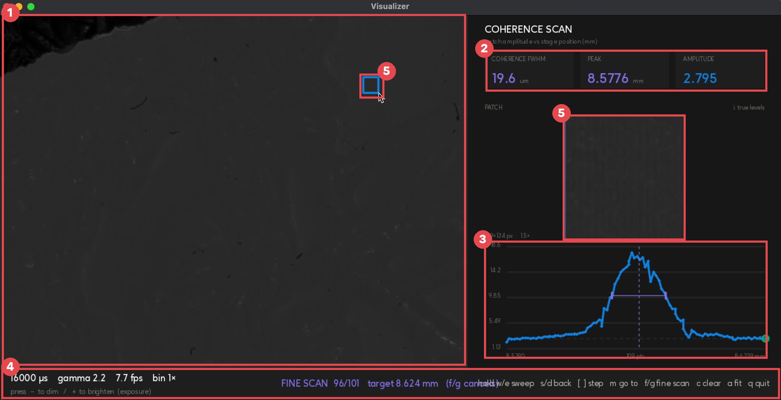
- ① Live camera view. The raw camera feed. Click twice on it to select a patch (first click anchors a corner, second finalizes).
- ② Stat tiles. Coherence FWHM and peak (filled in once a full envelope has been swept through) and the live amplitude of the selected patch.
- ③ Coherence plot. Builds up patch amplitude vs stage position as the stage moves. Scroll the mouse wheel over it to zoom, drag to pan.
- ④ Status bar. Exposure (µs), gamma, frame rate, and binning on the left; the current stage position and the coarse / fine step sizes in the middle; key hints on the right.
- ⑤ Selected patch. The blue box marks the patch whose interference amplitude the panel is tracking. The panel also shows that patch magnified, between the stat tiles and the plot, so you can see the fringes and speckle at sensor resolution instead of squinting at the small box on the live view. Press i if the fringes are too faint to make out.
Keyboard controls:
- w / s — jog the stage forward/back by the coarse step; hold w to sweep
- e / d — jog forward/back by the fine step (coarse ÷ 10); hold e for a slow sweep
- [ / ] — halve / double the coarse step size
- i — toggle auto-contrast on the magnified patch shown in the panel. The stretch
makes faint fringes visible, but it exaggerates contrast and hides how close you are to saturation —
the inset is labelled
i: auto-contrastwhenever it is on, so check that before you judge exposure - m — move to a position you type: press m, type the value in mm and press Enter (a leading + or - moves relative to where you are; Esc cancels). Handy for jumping straight back to a centre you found earlier
- + / - — brighten / dim (exposure)
- f — fine scan: once you have coarsely found the peak, steps ±0.5 mm around the current position in 10 µm steps (the plot resets as the sweep begins), saves a contrast-vs-position plot (PNG + CSV) and moves the stage to the peak
- g — refine scan: same as f but ±0.05 mm in 1 µm steps — run it after f has landed close, to polish the peak. Pressing f or g during a scan cancels it
- a — autoscale the plot (undo zoom/pan)
- c — clear the patch selection and the plot
- r — reset the plot but keep the patch
- q — quit
4Collimating the LED
- Set the lens to infinity focusing.
videoTurn the focus ring until the ∞ symbol sits over the index mark in the distance window (highlighted by the green box). - Adjust the telescoping tube until the images of the active element of the LED (this may look
different for each LED) look as sharp as possible.
Note: if you have the SM1NR1 telescoping tube, the LED should not rotate as you adjust it — only the tube extends. Some of the lens tubes (SM1U) do rotate as you turn them, so don't be alarmed if the LED spins with the adjustment on those.
videoSM1NR1 — the tube extends without rotating the LED. videoSM1U — the LED rotates with the adjustment. videoCollimating: the two images of the LED's active element sharpen up as the telescoping tube is adjusted. Note: LEDs come in different shapes, so don't expect yours to look like the one in the video — it just has to come into focus.Tip: You may choose to block one of the arms using a piece of card to make alignment easier.
5Making the mirrors parallel
Use the adjusters on the mirror mounts to position both images of the LED roughly at the center of the field of view of the camera (better aligned, the better). You can use the inset preview by selecting a crop region to help you align them precisely.
OCT
Now that we've collimated our light source and made the mirrors nearly parallel, we will now align it to use it for a time-domain OCT scanner: match the pathlengths of the two arms, measure the coherence length (your depth resolution), then scan an object and reconstruct its depth map.
1Coarse pathlength matching
- Focus the lens onto the object-side mirror. Block the mirror on the motorized stage using a piece of card. Change the lens focusing such that
the other mirror (straight opposite the camera) comes into focus (about 1:1).
videoChanging the lens focusing — turn the focus ring on the Nikon lens. videoBringing the mirror surface into focus at about 1:1 — watch the dust and scratches on the glass sharpen up. You will need to increase the exposure time and/or LED power.
Tip: Laterally move the mirror using the micro-adjusters until its edge comes into view, and make sure to focus on the edge — it gives you something sharp to judge the focus by. You may also use dust or scratches present on the mirror.videoLaterally translating the mirror with the stage's micro-adjuster to bring its edge into view. videoFocusing on the mirror's edge until it is sharp. - Unblock the mirror on the motorized stage. Leaving the lens focus setting fixed, adjust the stage position using the keys until this mirror comes into focus as well. You can use the same trick of laterally moving the mirror to bring its edge into view. The edge may not be perfectly at te same depth as the surface of the mirror, so try and refine it to focus on dust/scratches on the mirror. You should now have both mirrors in focus.
-
Now that both of the mirror arms are in focus, they are now coarsely matched to be at about the same distance from the beamsplitter. We now need to make this a lot more precisely matched (within the coherence length of the light source, typically
<40 µm) Select a patch on the live view — two clicks: the first anchors a corner, the second finalizes it. The coherence panel now tracks that patch as you move the stage.videoSelecting a patch: one click to anchor a corner, a second to finalize. If you're lucky, you may be able to perform precise alignment of the reference mirror (on the motorized stage) to match with the object-side mirror (right opposite the camera) using just the visualizer and using the w/s keys to move the stage. Most likely, you will need to automate the precise alignment, as described in the next step.What the panel is computing
The plotted value is the
computeMeanDiffmeasure: within the patch, take each frame's absolute deviation from the local (running) mean intensity, and average it — mean |I − DC|. The DC mean is the plain image; what's left is the amplitude of the interference fringes. That amplitude is essentially zero everywhere except when the two arms' pathlengths match to within the coherence length — so as you step the stage, the plot sits at a noise floor and then jumps in a sharp peak at the matched position. (Step 4 uses this same measure per-pixel to build the depth map.)
2Fine pathlength matching
- With a patch selected the f key runs a local scan centered around the current position of the stage— it covers a range of ±0.5 mm around the current position in 10 µm steps, then moves the stage to the peak and saves a contrast-vs-position plot.
- Once you've found a peak you should be able to see fringes already.
You can use the mirror-orientation adjusters to change the interference fringe pattern:
videoThe fringe pattern changing as the mirror-orientation adjusters are turned — the spacing and curvature of the fringes follow the relative tilt of the two mirrors. - Follow it with a scan with the g key to repeat the same kind of scan, but for a 10× finer range (±0.05 mm in 1 µm steps) and nail the centre to obtain peak fringe contrast.
3The temporal coherence length
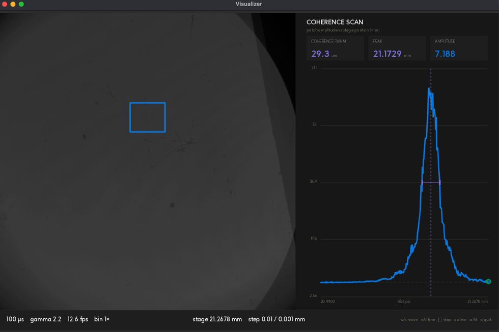
Performing a fine scan using either the f or g keys will give you a fully resolved coherence envelope. Find a saved plot of the interference contrast curve as a function of motor position in live_view_captures/.
The FWHM of this envelope is the temporal coherence length of the light source, which sets the depth resolution for OCT. You should also find it reported at the top panel of the visualizer window.
This temporal coherence length of the spectrally filtered light reaching the camera should be our depth resolution for OCT.
What should we expect?
The coherence length is set by the spectrum of the light: the wider the bandwidth, the faster the two arms decorrelate as their pathlengths separate. In terms of the frequency bandwidth Δf — or, more usefully here, the central wavelength λ and wavelength bandwidth Δλ —
L = cn Δf ≈ λ2n Δλ
with n = 1 in air. For our LED behind the 10 nm bandpass filter (λ ≈ 660 nm, Δλ ≈ 10 nm) this gives L ≈ (660 nm)² / 10 nm ≈ 44 µm. For a Gaussian spectrum the exact FWHM-to-FWHM relation carries an extra factor of 2 ln 2/π ≈ 0.44, i.e. L ≈ 19 µm — so a measured envelope FWHM of a few tens of microns (here ≈ 28 µm) is right where it should be. Without the filter, the LED's full ~25 nm bandwidth would cut this roughly in half — and some LEDs are much broader still (the 565 nm one, for example).
4Scanning a coin
- Now that we've aligned and characterized our OCT system, we're ready to scan objects! When you're ready, ask for a coin sample mount to swap in place of the
rectangular mirror, and mount a coin (quarter/euro/…) on it.
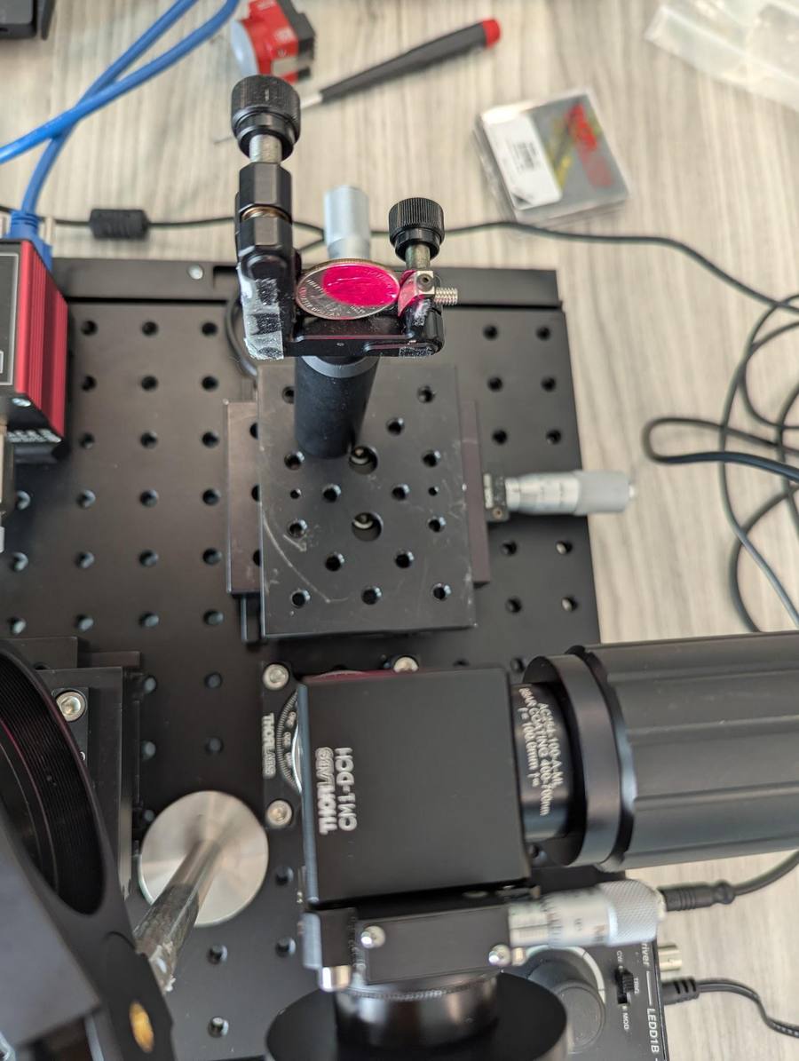
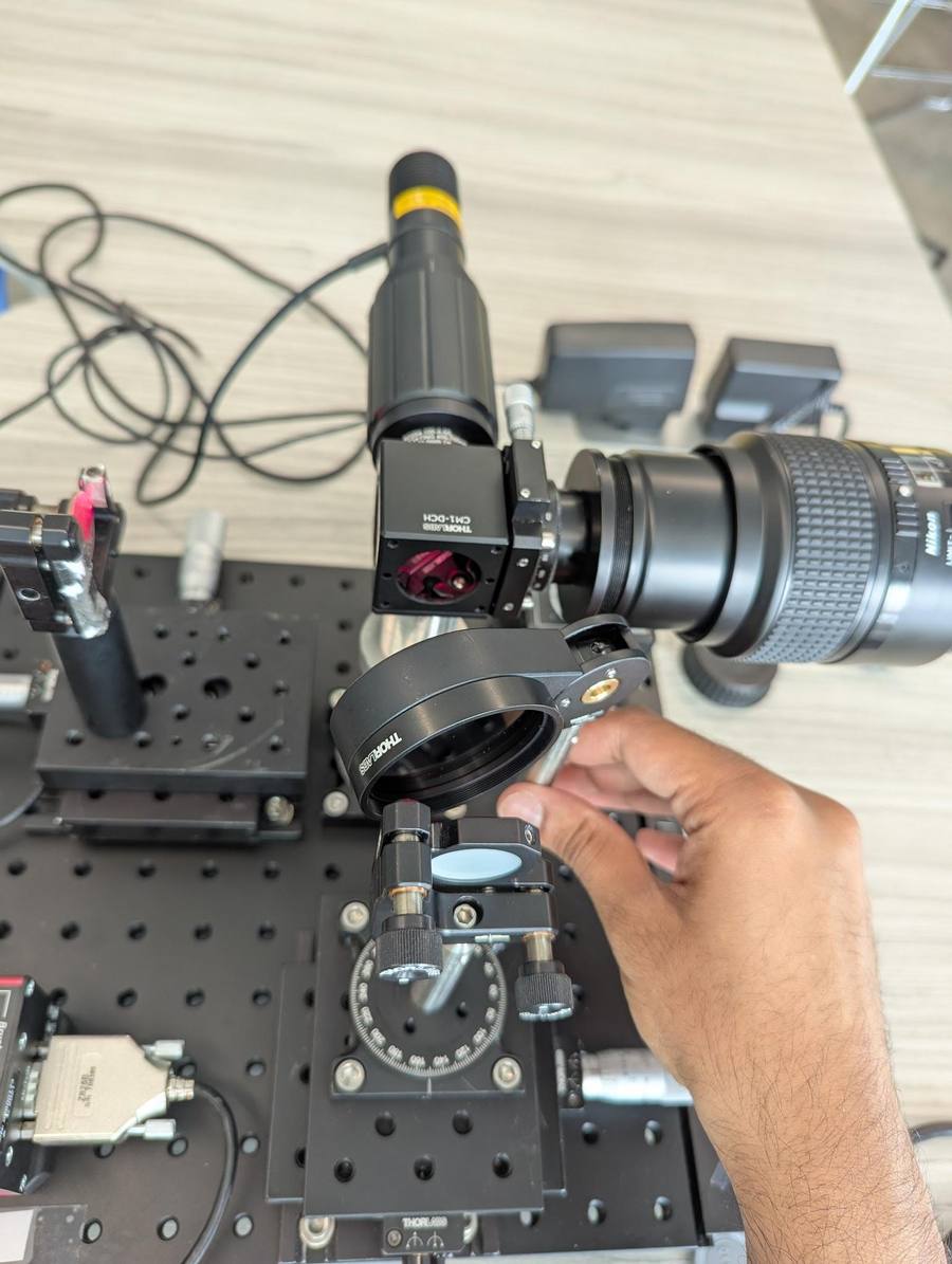
- Since the coin scattters light, it doesn't reflect all of the incident light back to the camera, and will appear much darker. Insert the 0.6 OD ND filter (placed at a slight angle to avoid inter-reflections) in the light
path to roughly match intensities from both arms. (You will need to readjust your exposure time.)
-
If we now scanned the reference arm through the entire range of the stage, we will be able to reconstruct a depth map of the coin based on when interference is detected at each region of the coin.
However, since the step size will need to be on the order of the coherence length (tens of microns), this would take nearly forever to complete.
Instead, we would like to align the reference mirror to a match the surface on a patch region on the coin using the same procedure that we followed for the mirror, and then do a short
1 mmOCT scan around that aligned position. -
To perform coarse alignment, leave the reference mirror and lens focusing fixed as it was before,
and bring the coin into
focus using its XY stage — turn the micro-adjusters until the coin's surface
detail is sharp in the live view. Just like we did for the mirror, we now have them coarsely matched, using the
fkey, we can automatically find the motor position that matches with the patch on the coin:- Press f for a coarse scan: it sweeps ±0.5 mm around the current position in 10 µm steps, plotting the patch contrast as it goes, and then tries to find a peak and moves the stage to it. When it lands you should see the speckle quite prominently in the patch — that's the coherence gate sitting on the coin's surface.
- Then, if you want to scan it better, press g for a fine scan: the same, but ±0.05 mm in 1 µm steps, to polish the peak position. (Pressing f or g again while a scan is running cancels it.)
videoPressing f: the coarse scan sweeps ±0.5 mm around the current position and lands on the coin surface's contrast peak. videoPressing g: the fine scan re-sweeps ±0.05 mm in 1 µm steps and resolves the full envelope around the peak. - Quit the visualizer, then perform a scan over a length of ~1 mm with
oct_scan.py. Use the temporal coherence length determined in step 3 to choose the step size — a few steps per FWHM, e.g. ~28 µm coherence → 5–10 µm steps. The captured stack may take a while to save. For the example below we used a 0.9 mm range with 3 µm steps, centred on the peak found above. The frame count is computed for you (range/step + 1), and if you leave out--exposurethe scan reuses the exposure from your last visualizer session (it is recorded inlast_exposure.jsonwhenever you adjust it):# 0.9 mm range x 0.003 mm steps = 301 frames, centred on the coherence peak # REPLACE the numbers with YOURS: --center is the peak position from the # coherence panel, --step-mm follows from YOUR measured coherence FWHM python oct_scan.py --center 12.3 --range-mm 0.9 --step-mm 0.003This saves a timestamped
stack_*.npyplus a*_meta.jsonsidecar with the scan geometry intooct_scans/.Caution:oct_scan.pysaves the stack as a.npythat is several GB in size (full resolution × hundreds of frames) — make sure you have disk space for it before starting the scan. - Run
oct_process.pyto recover a depth map from the scanned stack (it computes the mean-diff interference amplitude at every pixel and takes the depth of maximum contrast):python oct_process.py --stack oct_scans/stack_<timestamp>.npyTip: if you saved the stack at the original size and find the processing too slow, you can spatially downsample:python oct_process.py --stack oct_scans/stack_<timestamp>.npy -n 2 # -n 2 spatially downsamples 2x2 — purely to make the computation fasterIt saves
*_depth.npy,*_maxamp.npy, and a rendered*_render.png. To re-render with different color limits later, edit the settings at the top ofoct_view.pyand run it. A successful scan looks like this:
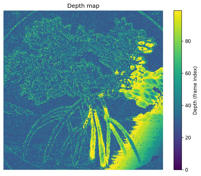
Depth map from a well-centred scan — the coin's relief is cleanly resolved over a smooth tilt gradient. (This coin is from another experiment, so it won't match the one in the photos above.) Caution: if your depth map looks like either of the ones below, part of the surface fell outside the scanned range — pixels clip at the first/last frame (flat saturated patches) or never see a peak at all (salt-and-pepper noise). Re-run the scan with a longer range and/or a better-centred start position.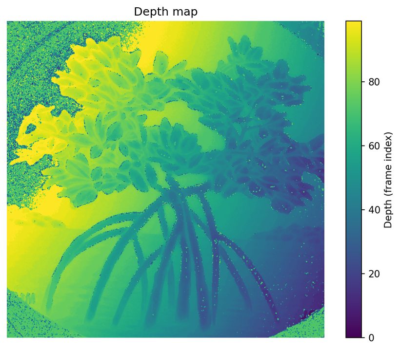
- (Optional) To see what the processing sees, render a side-by-side movie
of your scan with
oct_contrast_video.py: the raw captured frames on the left, and thecompute_mean_diffinterference amplitude |I − DC| on the right — the quantity whose per-pixel argmax becomes the depth map. Watch the bright band of contrast wash across the coin as the stage sweeps through each surface depth:python oct_contrast_video.py -s oct_scans/stack_<timestamp>.npy # -n 2 downsamples for speed; --fps and -o control the output movievideoRaw frames (left) vs interference amplitude (right) for a coin scan — the contrast band sweeping across the surface is the coherence gate crossing each pixel's depth; its per-pixel peak position is the depth map.
5Scanning other objects
Replace the coin with another object (or coin) of your choice and try doing the same!
depth_to_pointcloud.py converts a depth map
(plus its metadata sidecars) into a 3D point cloud you can inspect interactively.Software installations
The rig is a Thorlabs KDC101-driven motorized stage plus a monochrome machine-vision camera — either Allied Vision (via the Vimba X SDK) or IDS uEye (via pyueye). All the software runs from one Python environment.
1 · Getting the code
All the scripts live in the same repository as this page — github.com/cmu-ci-lab/summer-school — so if you're reading this locally, you already have them. If not:
git clone https://github.com/cmu-ci-lab/summer-school.git
cd summer-school
If fixes are posted during the course, git pull picks them up.
setup.sh will build a .venv instead.2 · Python environment: setup.sh
setup.sh prefers conda if you have it and falls back to a plain .venv if
you don't. On macOS run it from the Terminal; on Windows, run it from Git Bash (installed with
Git for Windows, which you likely already have):
chmod +x setup.sh
./setup.sh
# or, to force a venv even when conda exists:
FORCE_VENV=1 ./setup.shiccp-oct
environment is touched):
- creates or updates the
iccp-octenvironment fromenvironment.yml(Python 3.12, numpy, scipy, matplotlib, OpenCV, pyserial, pylablib, pyftdi); - searches the standard Vimba X install locations and installs the vmbpy wheel into the environment if the SDK is already present;
- on macOS, installs
libusb(conda-forge or Homebrew) — the stage backend; - registers a Jupyter kernel and prints the activation command for whatever it built.
3 · Alternative: manual conda install
If you'd rather not run the script and already have conda, create the environment directly from
environment.yml:
conda env create -f environment.yml
conda activate iccp-oct
(You'll still need to install your camera's SDK/bindings by hand — see step 5 below — and on
macOS the stage backend: conda install -c conda-forge libusb plus
pip install pyftdi.)
4 · Activating the environment
# conda path
conda activate iccp-oct
# venv path
source .venv/bin/activate        # Windows: .venv\Scripts\activate
In VSCode, pick the interpreter with Ctrl/Cmd+Shift+P →
Python: Select Interpreter → Python (iccp-oct) (or ./.venv). Some scripts
can also be run cell-by-cell in the Interactive Window, so it's worth setting this up now.
5 · Camera SDK & platform notes
This last step depends on your platform and on which camera your rig has — only one camera entry applies to you.
Windows
- Stage: install the Thorlabs Kinesis software from
thorlabs.com/software-pages/motion_control
(64-bit installer) — it provides the APT/FTDI driver (
ftd2xx.dll) that the KDC101 is detected through; without it the stage will not be found even though Python is set up correctly. Unplug/replug the KDC101 USB cable after installing. The Kinesis GUI is also handy for debugging — but close it before running the scripts, since it holds the controller exclusively. - Allied Vision camera:
vmbpyis not on PyPI — it ships as a wheel inside the Vimba X SDK. InstallVimbaX_Setup-2026-1-Win64.exe, then re-runsetup.sh(it finds and installs the wheel automatically), or install it yourself fromC:\Program Files\Allied Vision\Vimba X\api\python\vmbpy-*.whl. - IDS camera: two pieces — the
IDS Software Suite 4.97 for
Windows 32/64-bit (the native uEye SDK and driver; without it
pyueyeimports but every call fails), thenpip install pyueyeinto the project environment. If you're on IDS hardware you can skip Vimba X entirely; pass--camera idsto the hardware test so it doesn't check for vmbpy. Note: the IDS Software Suite has no macOS support — IDS cameras are Windows-only in this course (which is why the macOS section below has no IDS entry).
macOS
- Stage: no driver needed. Apple's FTDI driver ignores the KDC101's custom PID
(
0xfaf0), so no/dev/cu.usbserial-*port ever appears — don't hunt for one; the stage is driven directly over libusb viapyftdi.setup.shinstallslibusb(conda-forge or Homebrew) for you. - Allied Vision camera: install
VimbaX_Setup-2023-4-macOS.dmg, then re-runsetup.sh(it finds and installs the wheel automatically), or install it yourself from/Users/Shared/Allied Vision/Vimba X/Vmbpy/vmbpy-*.whl. - IDS camera: not supported on macOS (the IDS Software Suite is Windows-only in this course) — use a Windows laptop for IDS rigs.
python test_hardware.py: it searches the standard install
locations for you and prints the wheel's path along with the exact pip install command.iccp-oct or the venv first, then
pip install <path-to-vmbpy-*.whl>) — not into the system Python, or imports will
fail when you run from the project env.Troubleshooting
Plain python fails (a ModuleNotFoundError for pylablib,
cv2, vmbpy, … or the hardware suddenly "isn't found") — you're almost certainly running the
wrong Python: base conda, the system interpreter, or some other environment that happens to be
on your PATH. Two fixes:
- With the
iccp-octenvironment active, call its interpreter explicitly:"$CONDA_PREFIX/bin/python" visualizer.py - Or use the
./pythonwrapper that ships with the repo — it always resolves this project's interpreter (the activeiccp-octenv, then.venv, theniccp-octin the usual conda install locations), no matter what shell state you're in:./python visualizer.py ./python test_hardware.pyIf the wrapper is ever missing, a plain symlink to the env's interpreter does the same job:
ln -sf "$CONDA_PREFIX/bin/python" python
pip installs "succeed" but the import still fails — same root cause: bare
pip installed the package into whichever Python was on PATH, not the project env. Always
install through the same interpreter you run with:
./python -m pip install <package>
# equivalently:
"$CONDA_PREFIX/bin/python" -m pip install <package>
For hardware problems (stage or camera not found), re-run ./python test_hardware.py —
see step 1 of Part 2.